Useful R Commands

Published

February 16, 2026

Notebook 1: Basic R & Data Exploration

Assignment Operator (`<-`)

The assignment operator <- is used to store a value in an object.

Syntax

variable_name <- value

Example

# Store value 10 in x
x <- 10

# Print out value of x
x

[1] 10

`head()`

The head() function displays the first 6 rows of a dataset.

Syntax

head(dataset_name)

Example

head(dat)

    OPEID                                name       city state region
1  100200            Alabama A & M University     Normal    AL  South
2  105200 University of Alabama at Birmingham Birmingham    AL  South
3 2503400                  Amridge University Montgomery    AL  South
4  105500 University of Alabama in Huntsville Huntsville    AL  South
5  100500            Alabama State University Montgomery    AL  South
6  105100           The University of Alabama Tuscaloosa    AL  South
  median_debt default_rate highest_degree         ownership     locale hbcu
1      15.250         12.1       Graduate            Public Small City  Yes
2      15.085          4.8       Graduate            Public Small City   No
3      10.984         12.9       Graduate Private nonprofit Small City   No
4      14.000          4.7       Graduate            Public Small City   No
5      17.500         12.8       Graduate            Public Small City  Yes
6      17.671          4.0       Graduate            Public Small City   No
  admit_rate SAT_avg online_only enrollment net_price avg_cost net_tuition
1      89.65     959          No       5090    15.529   23.445       8.101
2      80.60    1245          No      13549    16.530   25.542      11.986
3         NA      NA         Yes        298    17.618   20.100      13.890
4      77.11    1300          No       7825    17.208   24.861       8.279
5      98.88     938          No       3603    19.534   21.892       9.302
6      80.39    1262          No      30610    20.917   30.016      14.705
  ed_spending_per_student avg_faculty_salary pct_PELL pct_fed_loan grad_rate
1                   4.836              7.599    70.95        75.04     28.66
2                  14.691             11.380    33.97        46.88     61.17
3                   3.664              4.545    74.52        84.93     25.00
4                   8.320              9.697    24.03        38.55     57.14
5                   9.579              7.194    73.68        78.05     31.77
6                   9.650             10.349    17.18        36.44     72.14
  pct_firstgen med_fam_income med_alum_earnings
1     36.58281        23.5530            36.339
2     34.12237        34.4890            46.990
3     51.25000        15.0335            37.895
4     31.01322        44.7870            54.361
5     34.34343        22.0805            32.084
6     22.57127        66.7335            52.751

`dim()`

The dim() function displays the dimensions (rows × columns) of a dataset.

Syntax

dim(dataset_name)

Example

dim(dat)

[1] 4435   26

The first number is the number of rows (horizontal), and the second is the number of columns (vertical).

`select()`

The select() function is used to select only certain variables (columns) from a dataset.

Syntax

new_data <- select(dataset_name, col1, col2, ...)

Example

example_dat <- select(dat, name, median_debt, ownership, admit_rate, hbcu)

`subset()`

The subset() function filters a dataset to obtain certain observations (rows), based on conditions.

Syntax

subset(dataset_name, condition)

Example

subset(example_dat, hbcu == "Yes" & admit_rate < 40)

                                               name median_debt
461                       Delaware State University      18.264
473                               Howard University      19.500
491  Florida Agricultural and Mechanical University      18.750
503                     Florida Memorial University      17.155
1376                        Alcorn State University      16.895
1401                                   Rust College      11.226
2747                             Hampton University      18.500
             ownership admit_rate hbcu
461             Public      39.34  Yes
473  Private nonprofit      38.64  Yes
491             Public      32.98  Yes
503  Private nonprofit      38.41  Yes
1376            Public      37.72  Yes
1401 Private nonprofit      29.47  Yes
2747 Private nonprofit      36.00  Yes

Common Conditions

Operator	Meaning	Example.
`==`	Equals exactly	`x == 10`
`!=`	Does not equal	`x != 10`
`<`	Less than	`x < 10`
`>`	Greater than	`x > 10`
`<=`	Less than or equal to	`x <= 10`
`>=`	Greater than or equal to	`x >= 10`
`\|`	Logical OR	`x < 5 \| x > 10`
`&`	Logical AND	`x > 5 & x < 10`

`arrange()`

The arrange() function orders the rows in a dataset based on one or more variables.

Syntax

arrange(data_name, column_name)

Example (ascending order)

arrange(example_dat, admit_rate)

                                         name median_debt         ownership
1                   Curtis Institute of Music      16.250 Private nonprofit
2                          Harvard University      12.072 Private nonprofit
3                         Stanford University      11.000 Private nonprofit
4                        Princeton University      10.355 Private nonprofit
5                             Yale University      12.000 Private nonprofit
6 Columbia University in the City of New York      19.250 Private nonprofit
  admit_rate hbcu
1       2.44   No
2       5.01   No
3       5.19   No
4       5.63   No
5       6.53   No
6       6.66   No

`desc()`

The desc() function modifies arrange() to put data in descending order.

Syntax

arrange(dataset_name, desc(column_name))

Example (descending order)

arrange(example_dat, desc(admit_rate))

                                                name median_debt
1 University of Arkansas Community College-Morrilton       6.250
2                      Design Institute of San Diego      31.000
3                                  Naropa University      16.390
4                        VanderCook College of Music      27.000
5                  Saint Elizabeth School of Nursing      20.291
6                 Maharishi International University      13.085
           ownership admit_rate hbcu
1             Public        100   No
2 Private for-profit        100   No
3  Private nonprofit        100   No
4  Private nonprofit        100   No
5  Private nonprofit        100   No
6  Private nonprofit        100   No

(`$`) operator

The $ operator selects a single variable (column) from a dataset.

Syntax

dataset_name$column_name

`table()`

The table() function displays frequency counts for the values of a categorical variable.

Syntax

table(dataset_name$column_name)

Example

table(dat$highest_degree)


 Associates   Bachelors Certificate    Graduate 
       1096         501        1374        1464

`gf_histogram()`

The gf_histogram() function creates a histogram of a quantitative variable.

Syntax

gf_histogram(~variable_name, data = dataset_name)

Example

gf_histogram(~admit_rate, data = dat)

Warning: Removed 2731 rows containing non-finite outside the scale range
(`stat_bin()`).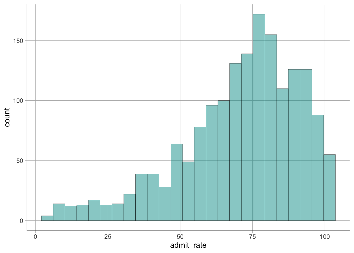

`gf_bar()`

The gf_bar() function creates a bar plot of a categorical variable.

Syntax

gf_bar(~variable_name, data = dataset_name)

Example

gf_bar(~highest_degree, data = dat)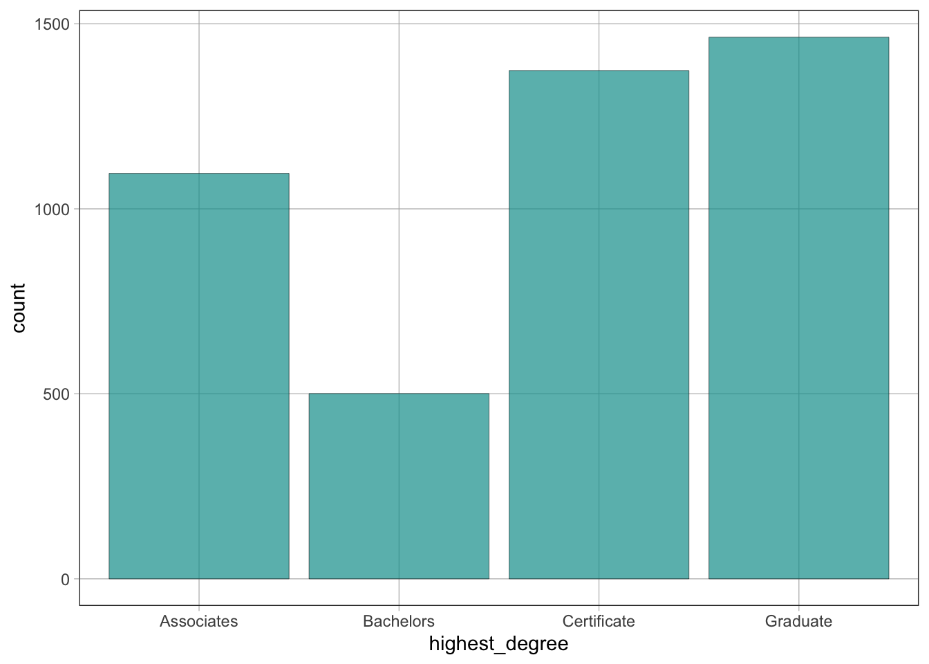

(`~`) Symbol

The ~ symbol is often used to separate the outcome variable ($y$) and predictor variable ($x$) in graphs and models:

outcome ~ predictor

`gf_boxplot()`

The gf_boxplot() function creates boxplots.

Syntax

gf_boxplot(outcome ~ predictor, data = dataset_name)

Example

gf_boxplot(admit_rate ~ highest_degree, data = dat)

Warning: Removed 2731 rows containing non-finite outside the scale range
(`stat_boxplot()`).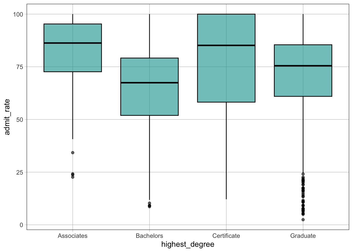

admit_rate ~ highest_degree means that admit_rate is the outcome ($y$) variable and highest_degree is the predictor ($x$) variable.
The boxplot displays admit_rate on the $y-$axis and highest_degree on the $x-$axis.

Notebook 2: Simple Linear Regression

(`~`) Symbol

The ~ symbol is used to separate the outcome ($y$) variable and the predictor ($x$) variable in graphs and models.

Syntax

outcome ~ predictor

Example

default_rate ~ pct_PELL

default_rate ~ pct_PELL

In this example, default_rate is the outcome ($y$) variable and pct_PELL is the predictor ($x$) variable.

`gf_point()`

The gf_point() function creates a scatterplot.

Syntax

gf_point(outcome ~ predictor, data = dataset_name)

Example

gf_point(default_rate ~ pct_PELL, data = dat)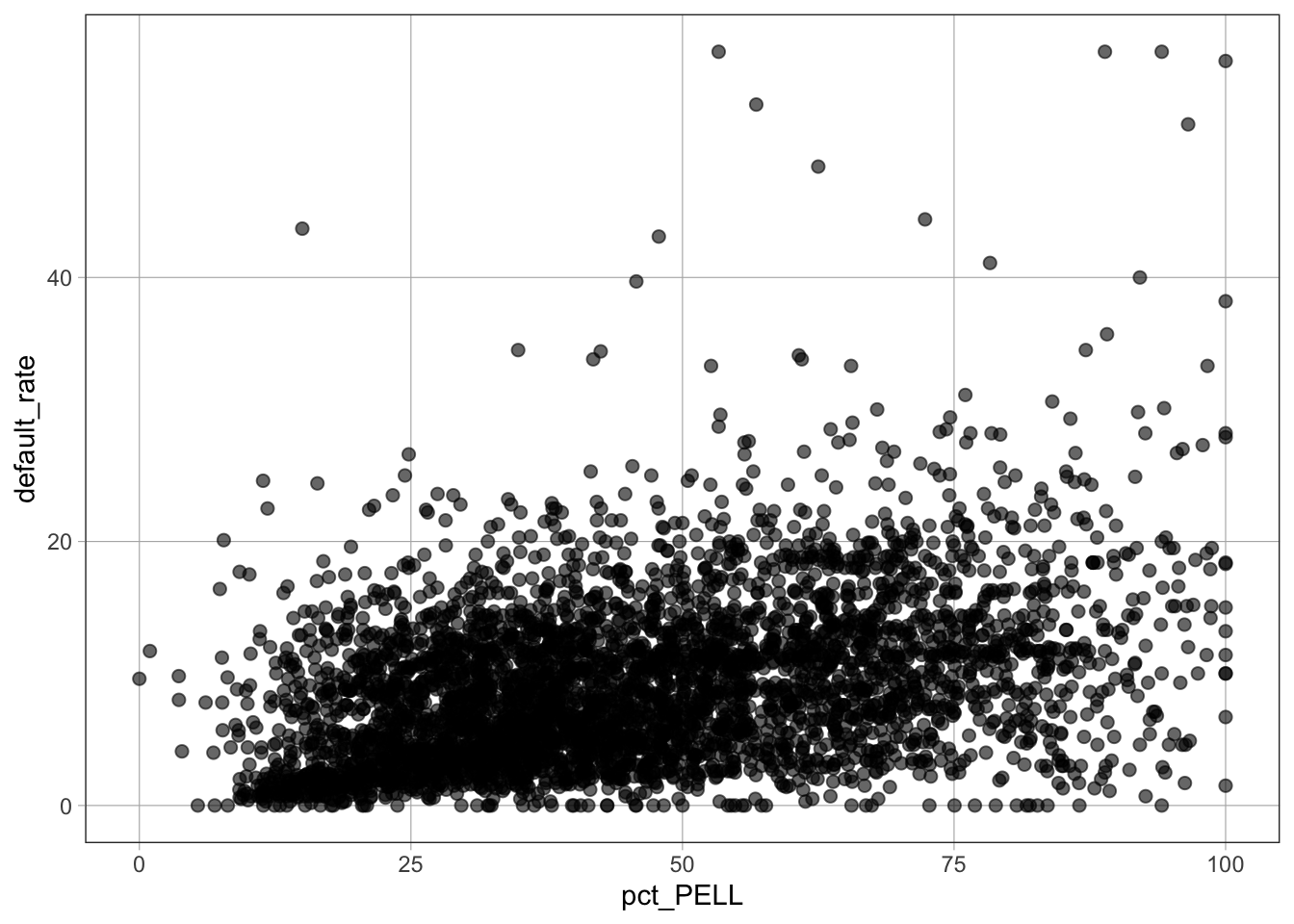

default_rate ~ pct_PELL specifies default rate on the $y$-axis and percent PELL on the $x$-axis
data = dat tells the function which dataset to use

(`%>%`) Pipe Operator

The %>% operator pipes the result of one command into the next command. It is often used to layer models on top of graphs.

Syntax

command_1 %>% command_2

Example

gf_point(default_rate ~ pct_PELL, data = dat) %>%
gf_lm(color = "orange")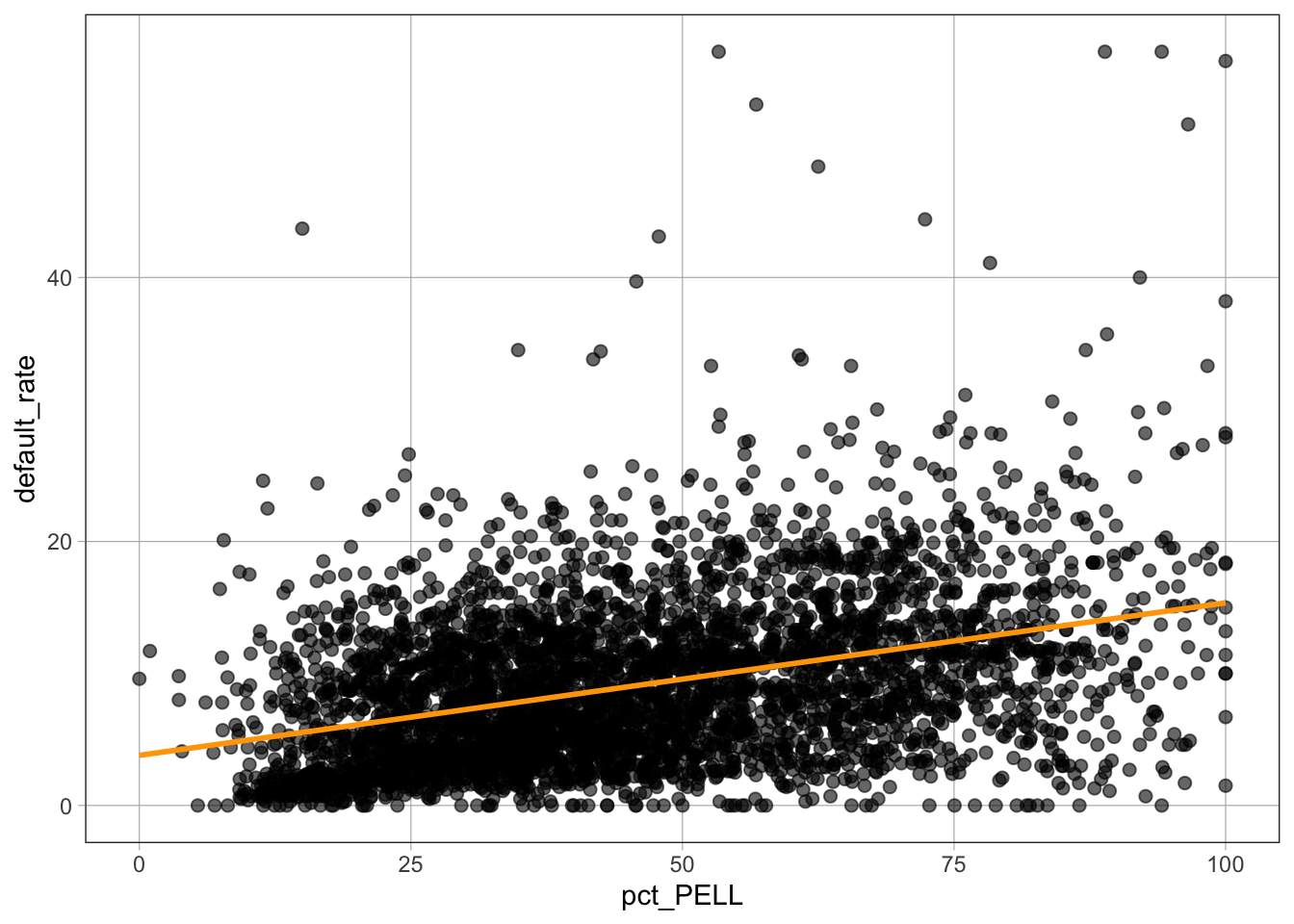

The first command creates the scatterplot
The second command overlays a linear model on top of the plot

`gf_lm()`

The gf_lm() function plots a linear model on an existing graph.

Syntax

gf_lm(color = "color_name")

Example

gf_point(default_rate ~ pct_PELL, data = dat) %>% 
  gf_lm(color = "orange")

color = "orange" sets the color of the fitted line

`lm()`

The lm() function fits a linear regression model.

Syntax

model_name <- lm(outcome ~ predictor, data = dataset_name)

Example

PELL_model <- lm(default_rate ~ pct_PELL, data = dat)
PELL_model


Call:
lm(formula = default_rate ~ pct_PELL, data = dat)

Coefficients:
(Intercept)     pct_PELL  
     3.7989       0.1155

default_rate ~ pct_PELL specifies the outcome and predictor
data = dat indicates the dataset used
PELL_model <- stores the model in an object named PELL_model
Printing the model displays the estimated coefficients

`summary()`

The summary() function displays detailed information about a fitted regression model.

Syntax

summary(model_name)

Example

summary(PELL_model)


Call:
lm(formula = default_rate ~ pct_PELL, data = dat)

Residuals:
    Min      1Q  Median      3Q     Max 
-14.669  -3.914  -0.974   3.113  47.142 

Coefficients:
            Estimate Std. Error t value Pr(>|t|)    
(Intercept)   3.7989     0.2095   18.14   <2e-16 ***
pct_PELL      0.1155     0.0042   27.50   <2e-16 ***
---
Signif. codes:  0 '***' 0.001 '**' 0.01 '*' 0.05 '.' 0.1 ' ' 1

Residual standard error: 5.68 on 4433 degrees of freedom
Multiple R-squared:  0.1457,    Adjusted R-squared:  0.1455 
F-statistic: 756.2 on 1 and 4433 DF,  p-value: < 2.2e-16

The output includes coefficient estimates and model statistics
Look for Multiple R-squared to find the $R^2$ value

Notebook 3: Multiple Regression

`lm()`

The lm() function can be used to fit a multiple regression model, where one outcome ($y$) variable is predicted using two or more predictors ($x_1, x_2, x_3, \ldots$).

Syntax

model_name <- lm(y ~ x1 + x2 + x3 + ..., data = dataset_name)

Example

tuition_grad_model <- lm(default_rate ~ net_tuition + grad_rate, data = dat)
tuition_grad_model


Call:
lm(formula = default_rate ~ net_tuition + grad_rate, data = dat)

Coefficients:
(Intercept)  net_tuition    grad_rate  
   13.04211     -0.18993     -0.03501

default_rate is the outcome ($y$) variable
net_tuition and grad_rate are predictor variables
The + symbol adds predictors to the model
data = dat tells R which dataset to use
tuition_grad_model <- stores the model in an object named tuition_grad_model

Running tuition_grad_model prints the estimated coefficients of the regression model.

`summary()`

The summary() function displays detailed information about a multiple regression model.

Syntax

summary(model_name)

Example

summary(tuition_grad_model)


Call:
lm(formula = default_rate ~ net_tuition + grad_rate, data = dat)

Residuals:
    Min      1Q  Median      3Q     Max 
-12.188  -4.049  -1.336   2.751  49.669 

Coefficients:
             Estimate Std. Error t value Pr(>|t|)    
(Intercept) 13.042108   0.238579  54.666  < 2e-16 ***
net_tuition -0.189926   0.012953 -14.663  < 2e-16 ***
grad_rate   -0.035014   0.004409  -7.941 2.52e-15 ***
---
Signif. codes:  0 '***' 0.001 '**' 0.01 '*' 0.05 '.' 0.1 ' ' 1

Residual standard error: 5.848 on 4432 degrees of freedom
Multiple R-squared:  0.09465,   Adjusted R-squared:  0.09424 
F-statistic: 231.7 on 2 and 4432 DF,  p-value: < 2.2e-16

Look for Multiple R-squared to find the $R^2$ value
Look for Adjusted R-squared to see the $R^2$ adjusted for the number of predictors

Notebook 4: Machine Learning

`poly()`

The poly() function adds polynomial terms to a regression model.

Syntax

poly(variable_name, degree)

Example

sat_model_2 <- lm(default_rate ~ poly(SAT_avg, 2), data = sample_dat)

sat_model_2


Call:
lm(formula = default_rate ~ poly(SAT_avg, 2), data = sample_dat)

Coefficients:
      (Intercept)  poly(SAT_avg, 2)1  poly(SAT_avg, 2)2  
            4.065             -8.391              4.355

default_rate is the outcome ($y$) variable
SAT_avg is the predictor ($x$) variable
poly(SAT_avg, 2) adds two polynomial terms: $x$ and $x^2$
data = sample_dat specifies the dataset used
sat_model_2 <- stores the fitted model in an object named sat_model_2

Running sat_model_2 prints the estimated coefficients of the polynomial regression model.

`predict()`

The predict() function generates predictions from a previously fitted model using new data.

Syntax

predict(model_name, newdata = dataset_name)

Example

predict(sat_model_2, newdata = test)

sat_model_2 is a previously fitted model
newdata = test specifies the dataset on which predictions are made
The output gives predicted values based on the model ```

Notebook 1: Basic R & Data Exploration

Assignment Operator (<-)

head()

dim()

select()

subset()

Common Conditions

arrange()

desc()

($) operator

table()

gf_histogram()

gf_bar()

(~) Symbol

gf_boxplot()

Notebook 2: Simple Linear Regression

(~) Symbol

gf_point()

(%>%) Pipe Operator

gf_lm()

lm()

summary()

Notebook 3: Multiple Regression

lm()

summary()

Notebook 4: Machine Learning

poly()

predict()

Assignment Operator (`<-`)

`head()`

`dim()`

`select()`

`subset()`

`arrange()`

`desc()`

(`$`) operator

`table()`

`gf_histogram()`

`gf_bar()`

(`~`) Symbol

`gf_boxplot()`

(`~`) Symbol

`gf_point()`

(`%>%`) Pipe Operator

`gf_lm()`

`lm()`

`summary()`

`lm()`

`summary()`

`poly()`

`predict()`